Subspace methods with asymptotic Krylov convergence for bounded variable problems.
Wim Vanroose, Bas Symoens
Abstract
Krylov subspace methods are highly effective in solving problems with sparse matrices at scale. Many large-scale problems in mechanics and fluid dynamics can be addressed using preconditioned Krylov solvers, and numerous specialized algorithms based on subspace methods have been developed that scale to the largest supercomputers. However, many scientific and engineering problems impose bounds on variables. Examples include nonnegative matrix factorization, contact problems in mechanics, and planning problems with resource and capacity constraints. Data science problems often have \(\|\cdot \|_\infty \)- or \(\|\cdot \|_1\)-norms. In these cases, active bounds manifest as boundary conditions, but it is often unknown in advance which bounds will be active.
Each bound on a variable is expressed as an inequality. In the optimality conditions, each inequality leads to a nonlinear complementarity condition that couples the variable and the corresponding Lagrange multiplier. The traditional approach is to linearize the system of optimality conditions and solve the resulting saddle point system. Each linearization is solved within a subspace with a iterative method for the saddle point problems [1]. However, this subspace is not reused in the next linearization; a new subspace is built in the subsequent outer iteration. This is inefficient.
We propose using a single subspace that is kept over all the iterations. Let us summarize how subspace methods reduce the problem and how we can generalize this.
A Krylov subspace for a square matrix \(A\in \mathbb {R}^{n\times n}\) and a vector \(v\in \mathbb {R}^n\) is defined as \(\mathcal {K}_k(A,v) := \text {span}\{v, Av, A^2 v, \ldots , A^{k-1}v \}\). Equivalently, this subspace can be written \(\text {span}\{r_0, r_1, r_2, \ldots , r_{k-1}\}\), where \(r_i\) are the residuals, which are mutually orthogonal.
The conjugate gradients methods (CG) minimizes the error in the \(A\)-norm over the Krylov subspace for a symmetric and positive definite matrix \(A\). Specifically, it solves \(\min _{x \in x_0 + \mathcal {K}_k(A,r_0)} \|x - x^*\|^2_A\). Expanding the solution as \(x_k=x_0+ V_k y_k\) and writing down the optimality conditions leads to a small linear system: \((V_k^T A V_k) y_k = \|r_0\|_2 e_1\). Since \(A\) is symmetric, the matrix \(V_k^T A V_k\) is a tridiagonal. If we have found the solution for a basis \(V_k\), the solution for the next iteration can be warm-started from the previous solution.
In the generalized minimal residual (GMRES), we minimize the 2-norm of the residual over the Krylov subspace. It is \(\min _{x \in x_0 + \mathcal {K}(A,r_0)} \|b-Ax\|_2\), for a general square matrix \(A\). The optimality conditions correspond to a small least-squares problem: \(\min _{y \in \mathbb {R}^k } \left \| \left \|r_0\right \|_2 e_1 -(V_{k+1}^TAV_k) y_k \right \|_2\). Here, the matrix \(V_{k+1}^T A V_{k}\) has a Hessenberg structure. Again, if we have found the solution for iteration \(k\), the next solution is easily found using warm-starting.
In this talk, we generalize this approach to a bounded variable least squares problem:
\(\seteqnumber{0}{}{0}\)\begin{equation} \label {eq:problem} \min \|Ax-b\|^2 \quad \text {subject to} \quad \ell \leq x \leq u, \end{equation}
where \(A \in \mathbb {R}^{m \times n}\), \(b \in \mathbb {R}^m\) and \(\ell ,u \in \mathbb {R}^n\), lower and upper bounds.
We will restrict the solution of (1) to a subspace, leading to a small projected problem. Instead of a small linear system as in CG or a small least-squares problem as in GMRES, this will now result in a small quadratic programming (QP) problem. This system will solve for the optimal coefficients of the solution and for the Lagrange multipliers. With these, we will calculate a residual that will be added to the basis.
Optimality conditions. Let us start with the optimality conditions for problem (1). These are
\(\seteqnumber{0}{}{1}\)\begin{equation} \label {eq:optimality} \begin{aligned} A^T(Ax-b) - \lambda + \mu &=0, \\ \lambda _i(x_i - \ell _i) &= 0, &&i\in \{1,\ldots ,m\}\\ \mu _i(u_i - x_i) &= 0, &&i\in \{1,\ldots ,m\} \\ \ell _i \leq x_i &\leq u_i, &&i\in \{1,\ldots ,m\}\\ \lambda \geq 0 \quad \mu &\geq 0. \end {aligned} \end{equation}
We now expand the solution in a orthogonal basis \(V_k\) as \(x_k = V_k y_k\). The problem (1) then becomes
\(\seteqnumber{0}{}{2}\)\begin{equation} \min \|A V_ky_k-b\|^2_2 \quad \text {subject to} \quad l \le V_k y \le u. \end{equation}
The corresponding optimality conditions are now:
\(\seteqnumber{0}{}{3}\)\begin{equation} \label {eq:projected_optimality} \begin{aligned} V_k^T\left ( A^T(A V_ky_k-b) - \lambda _k + \mu _k \right )&=0, \\ \lambda _i([V_ky_k]_i - \ell _i) &= 0, &&i\in \{1,\ldots ,m\}\\ \mu _i(u_i - [V_ky_k]_i) &= 0, &&i\in \{1,\ldots ,m\} \\ \ell _i \leq [V_ky_k]_i &\leq u_i, &&i\in \{1,\ldots ,m\}\\ \lambda \geq 0 \quad \mu &\geq 0. \end {aligned} \end{equation}
These are very similar to (2) but now the first equation is a projection of the residual onto the basis \(V_k\). The number of complementarity conditions is the same as in the original problem.
Residual Quadratic Programming Active Set Subspace (ResQPASS)). We are now in a position to define the ResQPASS iteration. It solves a series of small projected optimalisation problems that can be warm-started with the previous solution.
-
Definition 1. The residual quadratic programming active-set subspace (ResQPASS) [2] iteration for \(A \in \mathbb {R}^{m \times n}\), \(b \in \mathbb {R}^m\) and \(\ell ,u \in \mathbb {R}^n\), lower and upper bounds such that \(\ell \leq 0 \leq u\) with associated Lagrange multipliers \(\lambda _k, \mu _k \in \mathbb {R}^n\), generates a series of approximations \(\{x_k\}_{k \in \mathbb {N}}\) that solve
\(\seteqnumber{0}{}{4}\)\begin{equation} \label {eqn:xk} \begin{aligned} x_k = \argmin _{x \in \vct \{r_0,\ldots , r_{k-1}\}} & \|Ax-b\|_2^2 \quad \text {subject to} \quad \ell \leq x \leq u, \end {aligned} \end{equation}
where
\(\seteqnumber{0}{}{5}\)\begin{equation} \label {eqn:rk} r_k := A^T (Ax_k-b) - \lambda _k +\mu _k. \end{equation}
The feasible initial guess is \(x_0=0\), with \(\lambda _0=\mu _0=0\) and \(r_0 :=-A^Tb\).
The definition of the residual, (6), includes the current guess for the Lagrange multiplier \(\lambda _k\) and \(\mu _k\). A non-zero Lagrange multiplier indicates where the solution in the subspace touches the bounds.
Note that the residual, as defined in Eq. (6), also appears in the first equation of the optimality conditions, (2) and (4).
The restriction \(\ell \leq 0 \leq u\) does not limit the applicability, we can use an initial guess \(x_0\) to shift to problem such that this is satisfied.
This definition is translated in the algorithm described in Algorithm 1, which has a very similar structure as Krylov subspace methods.
Algorithm 1: Residual quadratic programming active-set subspace (ResQPASS)
-
Require: \(A \in \mathbb {R}^{m \times n},b \in \mathbb {R}^m\), \(\ell ,u \in \mathbb {R}^n, tol>0\)
-
1: \(r_0 =A^Tb\)
-
2: \(V_1 =r_0/\|r_0\|\)
-
3: \(y_1 = 0\)
-
4: \(\mathcal {W}_1 = \emptyset \)
-
5: for \(k=1,2,\ldots ,m\) do
-
6: \(y_k^*, \mathcal {W}_k^*,\lambda _k, \mu _k \gets \) Solve Eq. (4) using qpas, with initial guess \(y_k\) and initial working set \(\mathcal {W}_{k}\)
-
7: \(r_k = A^T\left (AV_ky_k^* - b\right )-\lambda _k+\mu _k\)
-
8: if \(\|r_k\|_2 \le tol\) then
-
9: \(x = V_k y_k,\) break;
-
10: end if
-
11: \(V_{k+1} \gets \begin {bmatrix} V_k & r_k/\|r_k\| \end {bmatrix}\)
-
12: \(y_{k+1} \gets \begin {bmatrix} (y_k^*)^T & 0 \end {bmatrix}^T\)
-
13: \(\mathcal {W}_{k+1} \gets \mathcal {W}_k^*\)
-
14: end for
If we solve the system of the projected optimality conditions (4) only to feasibility (i.e., not all Lagrange multipliers are positive), we obtain an orthogonal series of residuals \(r_k\). Indeed, the first equation of (4) shows the current residual projected on the previous residuals. Thus, achieving feasibility means that the current residual will be orthogonal to all previous residuals.
Another observation is that when the bounds, \(\ell \) and \(u\), do not restrict the problem (i.e none of the bounds are active), the corresponding Lagrange multipliers \(\mu \) and \(\lambda \) will be zero, due to the complementarity conditions. In this case, the residual simplifies to the classical form \(A^T(AV_ky_k-b)\), as in LSQR or CG. The method ResQPASS will then corresponds to a classical Krylov method.
However, when there are active bounds, the residuals will differ — but not significantly. When only a few bounds are active, the vectors of Lagrange multipliers are sparse, meaning that only a few of the elements \(\lambda _i\) and \(\mu _j\) are non-zero.
In figure 1, we studied model problems where the number of active constraints in the solution can be adjusted. What we observe is that, in the initial iterations, progress is slow because the bounds prevent a full step. However, once the limiting bounds are discovered, regular Krylov convergence sets in due to the orthogonality of the residuals.
This observation is explained by a convergence analysis [2], which reveals that after a certain number of iterations, the residuals can be expressed as polynomials of the normal matrix on some subspace, \(p(A^T A)V_0\). At this point, regular Krylov convergence occurs. This connection to Krylov subspaces suggests superlinear convergence for problems with a small number of active constraints.
Numerical implementation. In the numerical implementation, we solve a series of QP problems that grow in size. Similar to CG and GMRES, solving the next problem becomes easier if the previous problem has already been solved. We can warm-start with the previous solution as the initial guess, along with the working set from the previous problem. Additionally, the factorisation of the saddle point system can be reused, as the active set changes one element at a time, and the matrices only change by a rank-1 update.
We use a Cholesky factorization of the projected Hessian \(V_k^TA^TAV_k\) or a orthogonalisation \(AV_k=U_kB_k\), which gives asymptocally the bidiagonalisation. These factorisations ar efficiently updated as the subspace expands. Similarly, in the inner QP iterations, we use a QR factorization of the Cholesky factors applied to the active constraints, which further improves the efficiency.
By limiting the inner iterations we can choose to solve only for feasibility. In the early iterations, it is beneficial to prioritize subspace expansion over achieving full optimality within each subspace. This control over the number of inner iterations balances solution accuracy and speed. We also incorporate additional recurrence relations to avoid redundant computations, similar to techniques used in the CG method.
This results in an algorithm that performs very well in problems with a limited number of active constraints such as contact problems, offering significantly faster convergence compared to traditional methods like interior-point methods. However, the performance degrades as the number of active constraints becomes too large.
It is important to note that ResQPASS is a matrix-free method, as it primarily relies on matrix-vector products, making it suitable for problems where explicit matrix storage is impractical.
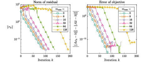
Figure 1: This figure illustrates the convergence behavior for different number of active constraints. The residual and objective behave similar to the unbounded (\(i_{\max }=0\), Krylov convergence) case, with a delay that is roughly equal to \(i_{\max }\), the number of active constraints in the problem. \(\tilde {x}\) is an ‘exact’ solution found by applying MATLAB’s quadprog with a tolerance of \(10^{-15}\).
References
-
[1] Michele Benzi, Gene H Golub, and Jörg Liesen. Numerical solution of saddle point problems. Acta numerica, 14:1–137, 2005.
-
[2] Bas Symoens and Wim Vanroose. ResQPASS: an algorithm for bounded variable linear least squares with asymptotic Krylov convergence. arXiv preprint arXiv:2302.13616, 2023.